Figure gallery
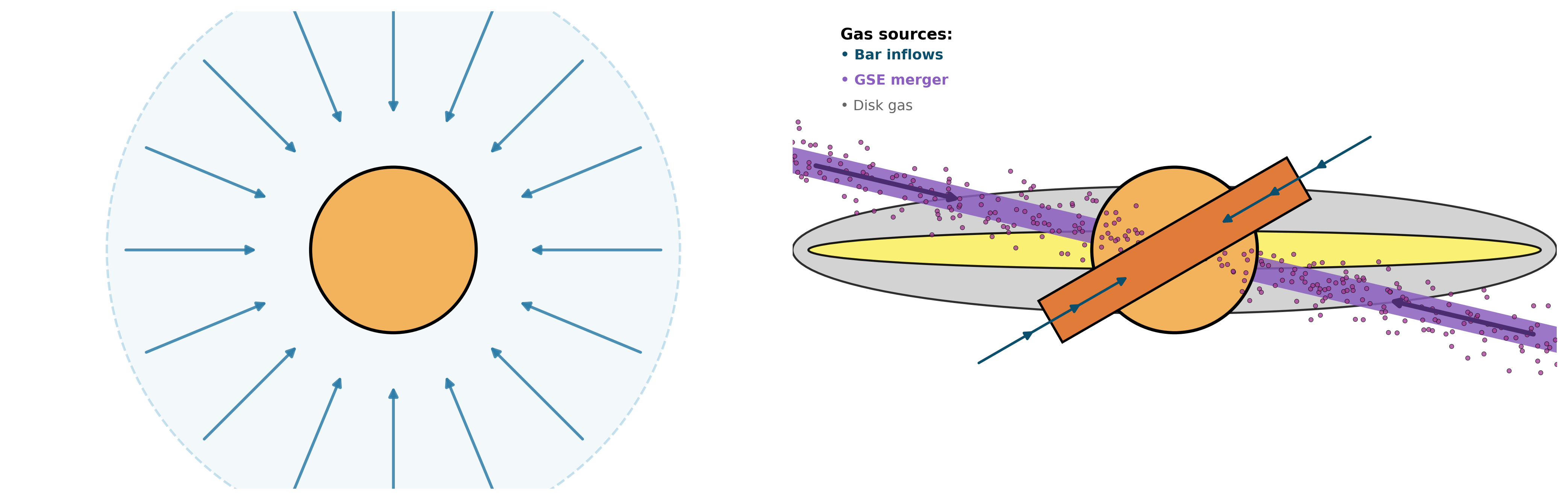
Schematic illustration of the two--infall framework used in this work. Left: Face-on (looking down the Galaxys rotation axis) view of the early bulge depicting the first infall (Shown by the blue arrows), represented as a rapid, centrally directed collapse that builds the classical bulge (Orange circle) in the absence of a bar or extended disk. Right: Diagonal view of the later galactic bulge during the second infall, where gas may be funneled inward along the existing bar (Orange rectangle) and disk (Yellow ellipse represents thin disk and grey ellipse represents thick disk), while additional material can arrive along more radial paths consistent with a GSE-like accretion event (Purple bar with red dots represents the GSE merger). All of the channels supply fuel to the same central region but differ in geometry and angular momentum, motivating the distinct evolutionary signatures explored in this study.
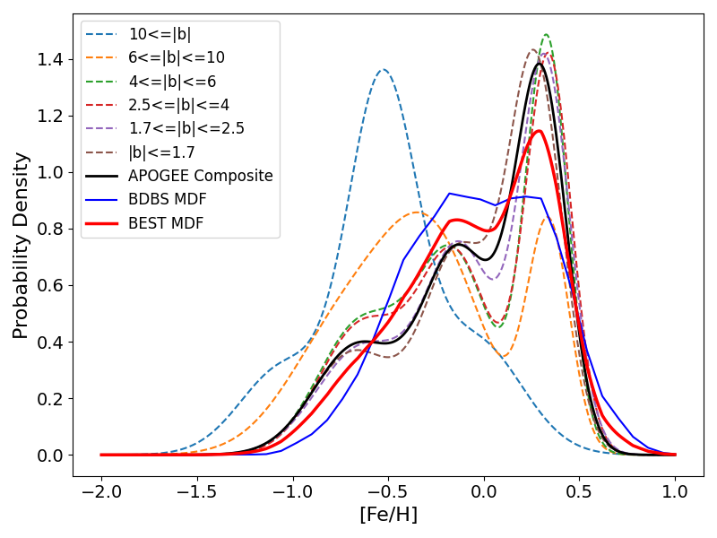
The figure shows the $\mathrm{[Fe/H]}$ distribution for the Milky Way bulge. Dashed lines indicate individual MDF fits from APOGEE DR16 across various Galactic latitude bands `$|\mathrm{b}|$'. The APOGEE Composite (thick black line) is the latitude-weighted average of the APOGEE fits. The BDBS MDF (blue line) is derived from red clump stars \citet{Johnson2022}. The composite MDF (thick red line) represents the final, equally-weighted composite observational target ($50\%$ APOGEE, $50\%$ BDBS) used for the Galactic Chemical Evolution (GCE) model optimization in this study. The target exhibits the characteristic bimodal distribution with peaks near $\mathrm{[Fe/H]} \sim -0.3$ and $\mathrm{[Fe/H]
Corner plot of posterior showing 1D histograms (diagonals) and 2D density (off–diagonals) continuous parameter groups. The black cross indicates the maximum \textit{a posteriori} (MAP). The red square highlights the Highest Density Interval (HDI)
Parameter dependency analysis. \textbf{Left:
Parameter dependency analysis. \textbf{Left:
Principal component analysis of the top-performing models. \textbf{Left:
Principal component analysis of the top-performing models. \textbf{Left:
Posterior corner plot for the continuous model parameters. Diagonal panels show 1D marginalized distributions with MAP (solid line) and 68\% highest–density intervals (dashed lines). Lower–triangle panels show the MDF–weighted model ensemble as a background point cloud with overlaid smoothed posterior density. The red crosses mark the MAP location in each 2D plane. Coloured stars and guide lines indicate parameter choices adopted in previous bulge studies, as listed in Table~\ref{tab:lit_results
Metallicity distribution function (MDF) of the bulge for the best-fit two-infall model compared to the observed MDF. In the upper panel, the blue shading shows the posterior predictive distribution of model MDFs as a function of $\mathrm{[Fe/H]}$, the red curve marks the single best-fit model realization, and the black crosses show the empirically measured, normalized MDF. The lower panel displays the residuals (model $-$ data) for the best-fit curve in each metallicity bin, with the overall root-mean-square residual of $\mathrm{RMS}=0.040$.
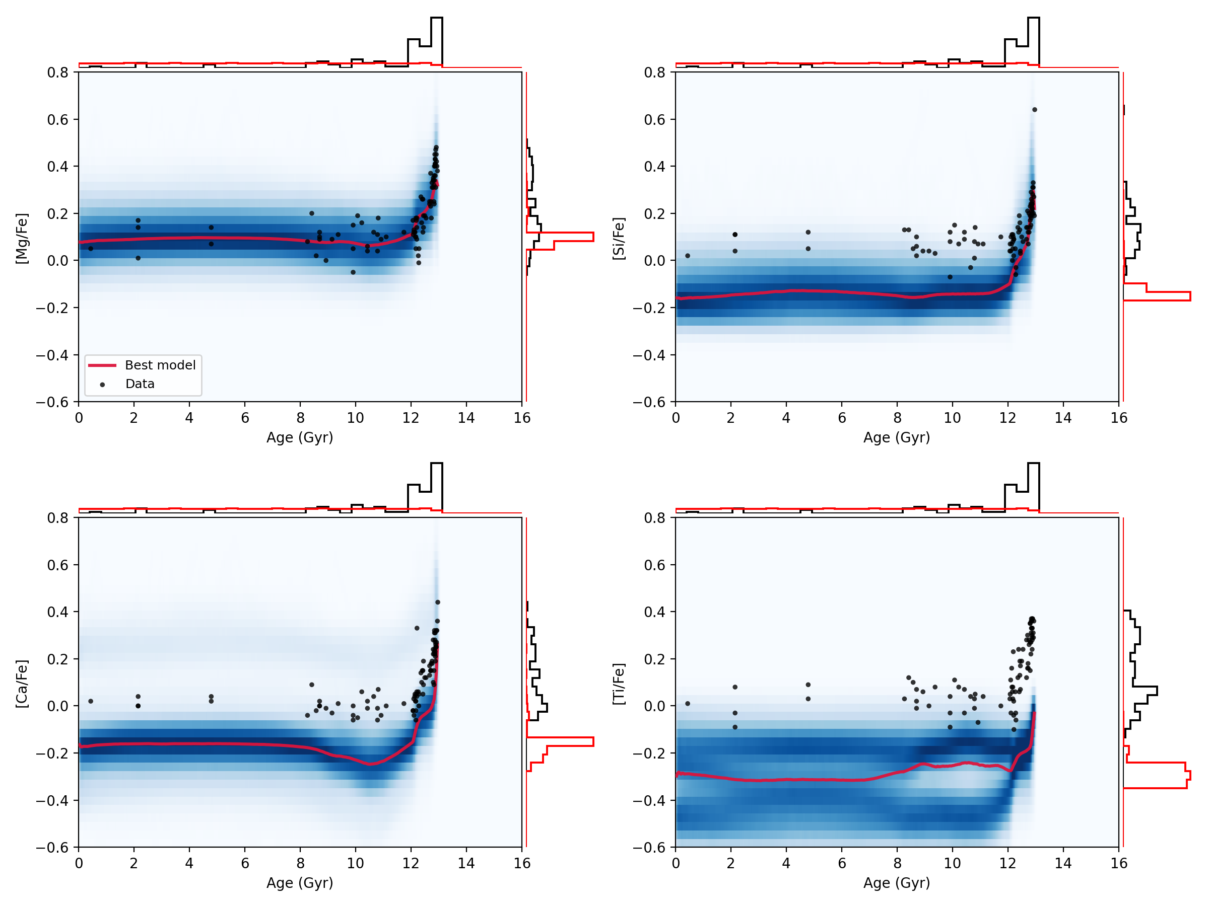
Posterior [$\alpha$/Fe]–[Fe/H] relations for individual bulge $\alpha$-elements Mg, Si, Ca, and Ti for the best-fit two-infall model. In each panel, blue shading shows the posterior predictive distribution of the model abundance ratios, the red curve traces the median (best-fit) model track, and black points indicate the observed stellar abundances. The top and right insets give the corresponding one-dimensional [Fe/H] and [$\alpha$/Fe] histograms for the data (black) and model (red).
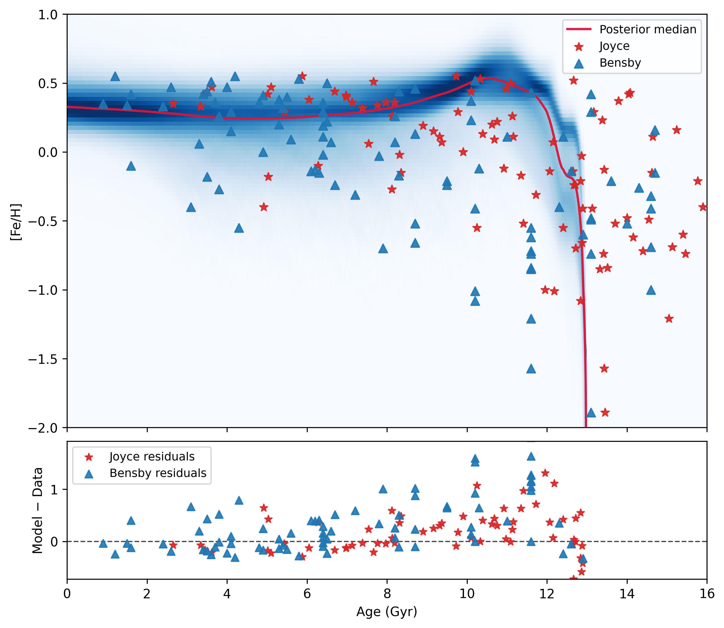
Posterior age–metallicity relation (AMR) for the bulge. The blue density field shows the weighted posterior ensemble of chemically acceptable models; the solid red line traces the MAP model. Individual stellar measurements are overplotted for comparison: \citet{Joyce2023} ages as red stars and \citet{Bensby17
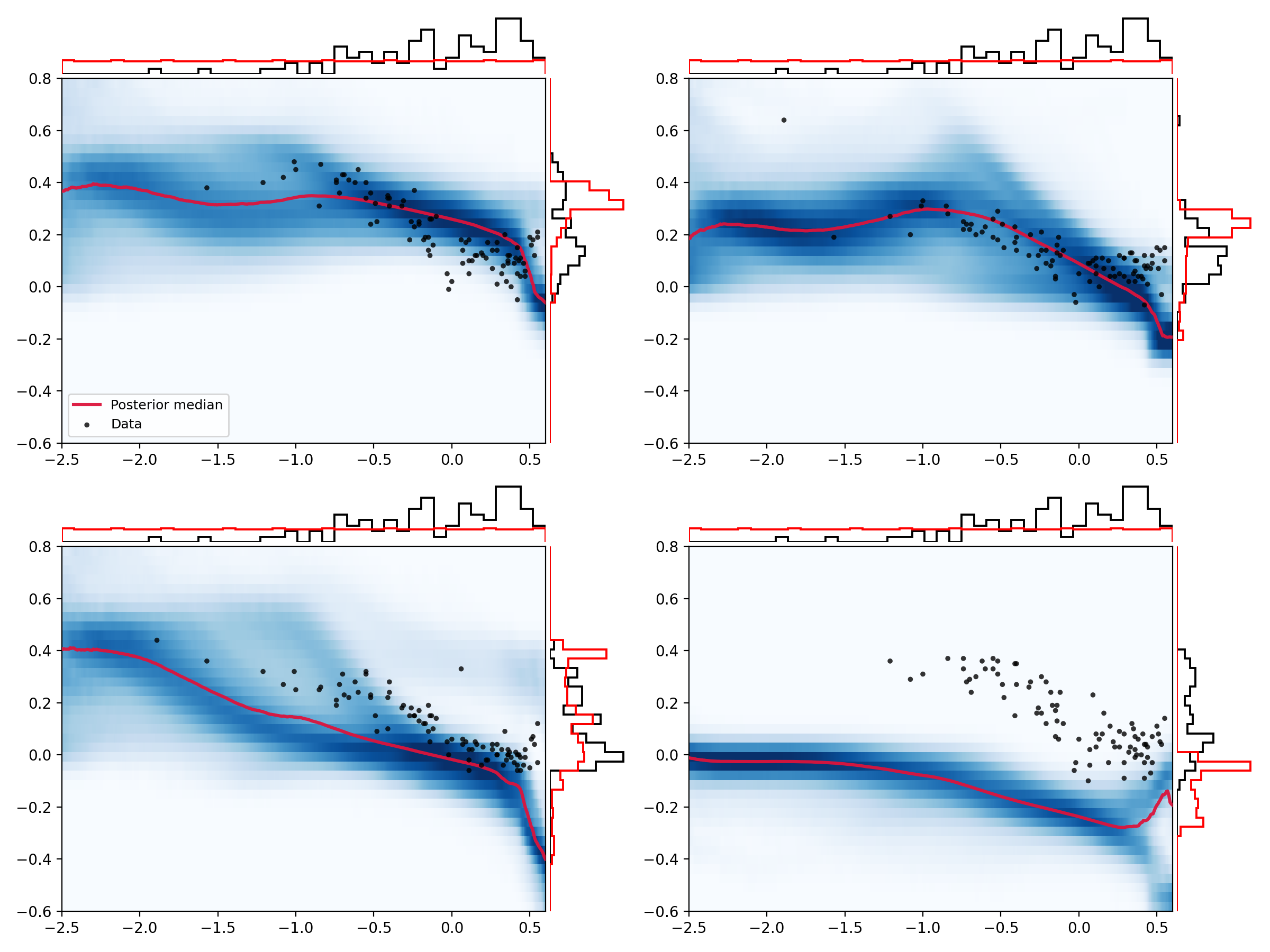
Posterior age--abundance relations obtained by mapping each model’s [$\alpha$/Fe]--[Fe/H] track through the median posterior age--metallicity relation. Blue shading indicates the weighted posterior density, and the solid red curve shows the best model. Observed bulge abundances are transformed into age using the same AMR mapping and shown as black points. The panels show the intermediate-age, metal-rich population suggested by the AMR occupies the low--[$\alpha$/Fe] sequence at ages $\sim 6$--$10$~Gyr, while the oldest stars remain on the high-[$\alpha$/Fe] plateau.
Corner plot of the joint posterior distribution in the continuous two–infall parameters obtained by combining 288 independent MCMC runs, one for each unique choice of categorical model ingredients Table~\ref{tab:parameter_space
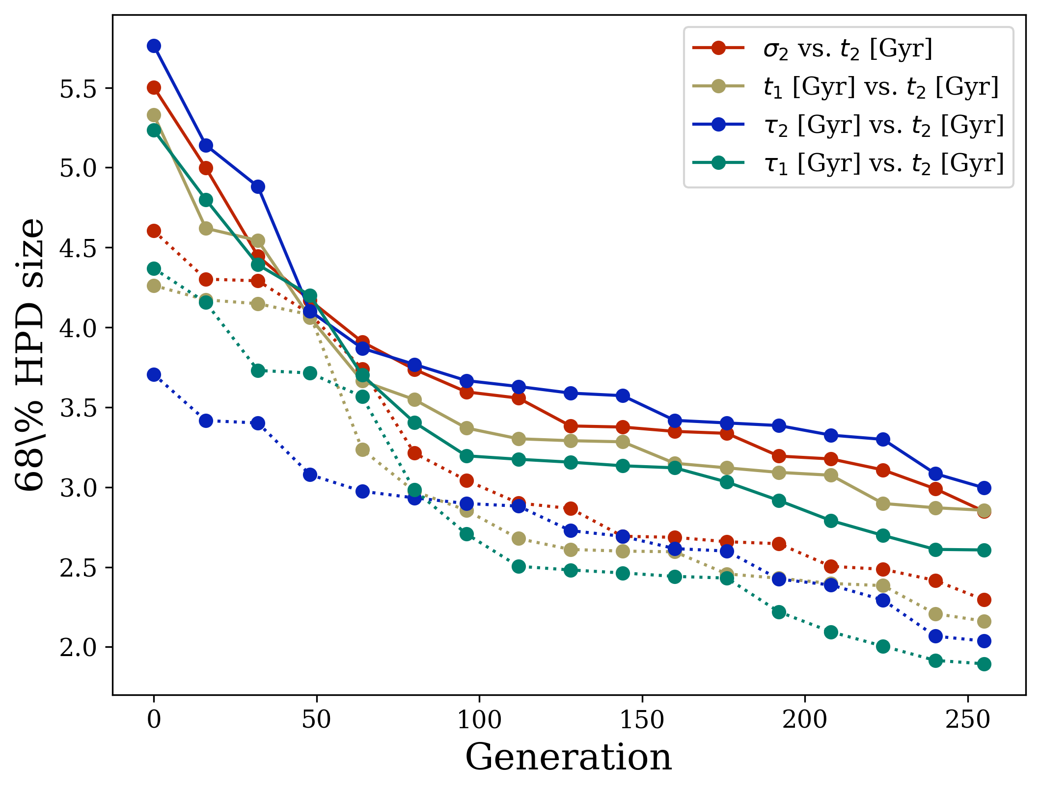
Convergence of the GA posterior. Solid lines show the evolution of the 68\% HPD ellipse size for several parameter pairs as a function of generation for a single GA run. Dotted lines show the corresponding HPD sizes measured from the combined pseudo–posterior used in the main corner plot. The rapid early decrease and subsequent plateau, together with the close agreement between solid and dotted curves, indicate stable and repeatable convergence of the GA.
Introduction
The Galactic bulge remains an archetype of composite stellar populations and overlapping formation channels. The bulge's formation history is complex and multifaceted, with various scenarios proposed in the literature. Previous works have suggested that the bulge formed primarily through a classical mechanism involving early mergers of primordial structures in a $\Lambda$ cold dark matter ($\Lambda$CDM) context \citep{Ortolani95, Baugh96, Abadi03a, Abadi03b}.
Schematic illustration of the two--infall framework used in this work. Left: Face-on (looking down the Galaxys rotation axis) view of the early bulge depicting the first infall (Shown by the blue arrows), represented as a rapid, centrally directed collapse that builds the classical bulge (Orange circle) in the absence of a bar or extended disk. Right: Diagonal view of the later galactic bulge during the second infall, where gas may be funneled inward along the existing bar (Orange rectangle) and disk (Yellow ellipse represents thin disk and grey ellipse represents thick disk), while additional material can arrive along more radial paths consistent with a GSE-like accretion event (Purple bar with red dots represents the GSE merger). All of the channels supply fuel to the same central region but differ in geometry and angular momentum, motivating the distinct evolutionary signatures explored in this study.
Manuscript excerpt (raw LaTeX lines)
The Galactic bulge remains an archetype of composite stellar populations and overlapping formation channels.
The bulge's formation history is complex and multifaceted, with various scenarios proposed in the literature.
Previous works have suggested that the bulge formed primarily through a classical mechanism involving early mergers of primordial structures in a $\Lambda$ cold dark matter ($\Lambda$CDM) context \citep{Ortolani95, Baugh96, Abadi03a, Abadi03b}.
Others have argued for a secular origin, where the bulge arises from disk instabilities and bar formation \citep{Combes90, Raha91, ONeill03, Athanassoula05, Shen10, Ciambur21, Ghosh23}.
More recent studies have proposed hybrid scenarios, combining an initial rapid collapse with later bar-driven evolution \citep{McWilliam10, Wegg13, Ness16, Barbuy18}.
Barred regions often exhibit flattened age and metallicity gradients compared to their disks \citep{Fraser2020, Neumann2020, Seidel2016}.
Structurally, the bulge shows evidence of both a boxy/peanut bar and a classical spheroid \citep{Barbuy18, Weiland94, McWilliam10, Wegg13, Ness16}.
Chemically, the bulge exhibits a broad metallicity distribution with distinct $\alpha$-enhancement patterns, motivating two-component formation scenarios \citep{Babusiaux10, Gonzalez11, Bensby11, Hill11, Uttenthaler12}.
The metallicity distribution function (MDF) of the bulge is characterized by a multi-peak shape, often bimodal, with a metal-poor peak centered at [Fe/H] $\sim -0.3$ dex and a metal-rich peak at [Fe/H] $\sim +0.3$ dex \citep{Bensby11, Hill11}.
This bimodality is also reflected in the [$\alpha$/Fe] versus [Fe/H] abundance ratios, suggesting the presence of different stellar populations --- a metal-poor population with spheroid kinematics and enhanced [$\alpha$/Fe] ratios, indicative of rapid formation, and a metal-rich one with bar-like kinematics and near-solar [$\alpha$/Fe], possibly originating from the inner disk \citep{Rich90,Rich1990,Matteucci90,Minniti1996, McWilliam94, Valenti05}.
The bulge’s MDF bimodality, the split in its $\alpha$-element trends, and the coexistence of old $\alpha$-enhanced stars with a younger, metal-rich population all imply at least two chemically distinct enrichment phases.
These observational features cannot be reproduced by a single rapid star-formation event, motivating models with multiple, temporally separated gas-accretion episodes \citep[e.g.,][]{Matteucci19, Molero2024}.
Modelling the bulge formation history as a two-infall process is a natural framework to explore these complexities.
While the two-infall paradigm was originally developed in the context of the Galactic disk, its conceptual structure remains useful when applied to the bulge, and so we draw on those disk-based studies for methodological guidance.
In this paradigm, an early rapid infall (producing $\alpha$-rich stars) is followed by a slower, prolonged phase of star formation (producing more Fe-rich stars).
Subsequent studies refined the two-infall scenario to reproduce abundance data across the disk (e.g., \citealt{Chiappini2001, Chiappini2003, Griffith2021}).
Others have explored the supernova Ia (SN\,Ia) delay-time distribution \citep{Matteucci09, Palicio23}, galactic fountains \citep{Spitoni09}, radial gas flows variations in the star formation efficiency (SFE) \citep{SpitoniMatteucci11}, radial stellar migration \citep{Morossi15}, azimuthal abundance variations \citep{Spitoni2019}, and pre-enriched gas infall \citep{Jacquier24}.
\citet{Palla24} proposed a third gas accretion event in the last $\sim 3$ Gyr to match the inferred star formation history from Gaia \citep{Ruiz18} and to explain the recent abundance evolution (or lack thereof) in the Solar neighborhood.
This picture is connected to the broader, currently accepted view of Milky Way formation.
The Galaxy consists of a central bulge; a thick disk, which has a larger scale height and shorter radial extent; a thin disk, where stars have smaller vertical dispersions and ongoing star formation; and a halo made up of old stars from the Milky Way as well as accreted stars from a variety of dwarf galaxy mergers \citep{Fuhrmann98, McWilliam03, Sara}.
Works tend to agree that the kinematically and spatially thick disk overlaps significantly with the stars formed early in the galaxy's history, where Type II supernovae had significantly enriched the gas in $\alpha$-elements, but Type Ia supernovae had not yet had sufficient time to add large numbers of iron-peak elements \citep{Tinsley79, Matteucci1986, Matteucci09, Kobayashi2011}.
These stars are therefore enhanced in $\alpha$-elements and are generally old, although debate is still ongoing about whether these stars started forming almost 14 Gyr ago, shortly after reionization, or there was a delay until about 10 Gyr ago, as well as whether there was a sharp burst of formation, or a more continuous process \citep{Aguirre2018, Xiang2022}.
Around $\sim 8$--$11$~Gyr ago, the galaxy associated with the Gaia--Enceladus Sausage (GSE) merged with the Milky Way \citep{Myeong2018, Lane2023, Liu2024, Kim2021, Belokurov2018}.
This system is thought to have been roughly one tenth the mass of the Milky Way at that time, and as such brought in a significant number of stars, now generally moving retrograde through the stellar halo. Furthermore, it potentially introduced a large amount of unprocessed gas \citep{Kordopatis2020} that altered the chemistry of stars formed after this time.
More recently formed stars are generally associated with the physically and kinematically thin disk.
These stars tend to have iron-rich and $\alpha$-poor compositions, and the combination of chemical and age information has suggested that star formation and chemical enrichment proceeded more rapidly in the inner Galaxy and more slowly in the outer galaxy \citep{Hayden15, Nidever24}. There is also strong evidence that significant numbers of stars migrate radially through the galaxy, changing their galactocentric radii and sometimes their height above the plane \citep{Schonrich09, Kubryk15, Sharma21}.
Today, we see that the Galactic bar, and the interactions between the bar and the disk, funnel stars and gas from the disk into the bulge \citep{Binney91, Bissantz02, Lopez05}. While it is challenging to work back in time, and bars in galaxies tend to be transient or short-lived features \citep{Tacchella15, Nelson16}, it is possible or even likely that these significant events in the broader Galaxy may have affected the star formation in the bulge, representing additional peaks in star formation at particular times and durations with particular compositions \citep{Elmegreen99, McWilliam03, Sara}.
Recent re-analyses of microlensed bulge dwarfs challenge this picture. In particular, \citet{Joyce2023} recompute ages for the \citet{Bensby17} microlensed sample using customized MESA Isochrones \& Stellar Tracks (MIST)-based isochrones and find an age--metallicity distribution that is markedly older and narrower than previous findings \citep{Bensby17}. Furthermore, the field of Galactic archaeology has advanced through large-scale spectroscopic surveys such as Gaia-ESO \citep{Gilmore12}, and APOGEE \citep{Majewski17}, providing detailed abundance patterns that demand comprehensive GCE models to interpret \citep{Ballero07, Grieco12, Molero2024, Dubay2025}.
To guide the interpretation of our model assumptions, Figure~\ref{fig:intro-cartoon} summarizes the geometric and physical structure of the two–infall framework adopted in this work.
The left panel represents the initial, rapid collapse phase that builds the classical bulge, characterized by centrally concentrated gas inflows without a pre-existing bar or extended disk.
Observational Data
The primary optimization target is a composite MDF combining data derived from red clump stars via the Blanco DECam Bulge Survey \citep{Johnson2022} and a parameterization of the RGB-based APOGEE DR16 MDFs at various latitudes provided by \citet{Rojas2020}. The latter data set is included primarily to improve coverage at the metal-poor ([Fe/H] $<$ $-1$) end, which is not well-sampled by red clump stars in \citet{Johnson2022}. The two data sets were normalized by applying a latitude-based weighting of source counts based on the equation: where $\frac{N}{N_{o}}$ represents the fraction of stars observed at a given Galactic latitude ($b$). The scaling relation is based on a fit to the latitude-dependent angular mass density relation at $l$=0 provided by \citet{Zoccali2018}. The BDBS data were interpolated onto the APOGEE [Fe/H] grid, and the final composite MDF is shown in Figure~\ref{fig:best_mdf}. We note that the BDBS distribution (derived from Red Clump stars) appears less visually bimodal than the APOGEE distribution (derived from RGB stars). This difference likely stems from the distinct selection functions and tracer sensitivities of the two surveys.
The figure shows the $\mathrm{[Fe/H]}$ distribution for the Milky Way bulge. Dashed lines indicate individual MDF fits from APOGEE DR16 across various Galactic latitude bands `$|\mathrm{b}|$'. The APOGEE Composite (thick black line) is the latitude-weighted average of the APOGEE fits. The BDBS MDF (blue line) is derived from red clump stars \citet{Johnson2022}. The composite MDF (thick red line) represents the final, equally-weighted composite observational target ($50\%$ APOGEE, $50\%$ BDBS) used for the Galactic Chemical Evolution (GCE) model optimization in this study. The target exhibits the characteristic bimodal distribution with peaks near $\mathrm{[Fe/H]} \sim -0.3$ and $\mathrm{[Fe/H]
Manuscript excerpt (raw LaTeX lines)
The primary optimization target is a composite MDF combining data derived from red clump stars via the Blanco DECam Bulge Survey \citep{Johnson2022} and a parameterization of the RGB-based APOGEE DR16 MDFs at various latitudes provided by \citet{Rojas2020}.  The latter data set is included primarily to improve coverage at the metal-poor ([Fe/H] $<$ $-1$) end, which is not well-sampled by red clump stars in \citet{Johnson2022}.  The two data sets were normalized by applying a latitude-based weighting of source counts based on the equation:
\begin{equation}
\frac{N}{N_{o}}=1.029e^{0.476\cdot b}
\end{equation}
where $\frac{N}{N_{o}}$ represents the fraction of stars observed at a given Galactic latitude ($b$).  The scaling relation is based on a fit to the latitude-dependent angular mass density relation at $l$=0 provided by \citet{Zoccali2018}.  The BDBS data were interpolated onto the APOGEE [Fe/H] grid, and the final composite MDF is shown in Figure~\ref{fig:best_mdf}.
We note that the BDBS distribution (derived from Red Clump stars) appears less visually bimodal than the APOGEE distribution (derived from RGB stars). This difference likely stems from the distinct selection functions and tracer sensitivities of the two surveys.
Methodology
The One-zone Model for the Evolution of Galaxies and Abundances (OMEGA) \citep{Cote2016}\footnote{\url{https://github.com/NuGrid/NUPYCEE}} is a single-reservoir chemical evolution framework that follows the time-dependent enrichment of a well-mixed galactic gas zone. In its baseline configuration, OMEGA assumes instantaneous mixing within a single gas reservoir and evolves the chemical composition under global prescriptions for star formation, stellar ejecta, and gas accretion. We incorporate nucleosynthetic yields through the SYGMA/NuPyCEE\footnote{\url{https://nugrid.github.io/NuPyCEE/}} framework.
Manuscript excerpt (raw LaTeX lines)
\subsection{Galactic Chemical Evolution Modeling Framework}
The One-zone Model for the Evolution of Galaxies and Abundances (OMEGA) \citep{Cote2016}\footnote{\url{https://github.com/NuGrid/NUPYCEE}} is a single-reservoir chemical evolution framework that follows the time-dependent enrichment of a well-mixed galactic gas zone.
In its baseline configuration, OMEGA assumes instantaneous mixing within a single gas reservoir and evolves the chemical composition under global prescriptions for star formation, stellar ejecta, and gas accretion.
We incorporate nucleosynthetic yields through the SYGMA/NuPyCEE\footnote{\url{https://nugrid.github.io/NuPyCEE/}} framework.
For massive stars ($M_{\star} \gtrsim 8\,M_{\odot}$), each GCE model adopts \emph{one} of several alternative massive–star yield grids: the rotating models of \citet{Limongi2018}, the non–rotating models of \citet{Limongi2018}, or the Nomoto/Chieffi SN\,II and hypernova–enabled grids \citep{Nomoto2013,Chieffi2013}.
These massive–star yield sets are treated as distinct categorical ingredients in our model grid, and no model combines more than one massive–star yield set.
Enrichment from low– and intermediate–mass stars ($M_{\star} < 8\,M_{\odot}$) is taken from the Monash yields of \citet{Karakas2010}.
Type~Ia supernova enrichment uses the metallicity–dependent yields of \citet{Shen2018} and \citet{Gronow2021}, coupled to several standard delay–time distributions (power–law, Gaussian, and exponential) following \citet{Greggio2005,Strolger2004,Matteucci2001,Maoz2014}.
These SN\,Ia prescriptions constitute an additional categorical dimension in the model grid.
The initial chemical composition of gas --- both at the start of the simulation and for any newly accreted inflow --- is drawn from the STELLar ABundances (STELLAB) library provided by NuPyCEE. \citep{Pignatari2016, Ritter2018, Battino2019}  This library consists of observed stellar abundance patterns (i.e.\ real-ISM / stellar-population abundances across elements) rather than pure primordial (H + He) composition.
Thus, inflowing material is initialized with non-zero metallicity values representative of interstellar/circum-galactic gas, as inferred from observations.
All chemical enrichment occurs in a single, well mixed bulge gas reservoir.
Gas flows (inflow or outflow) simply add to or remove mass from this same reservoir, with instantaneous mixing and a homogeneous chemical composition throughout.
An extended version of OMEGA, OMEGA+ \citep{Cote2018, Cote2019}, was designed to model multi-phase and multi-episode galactic evolution.
OMEGA+ introduces a chemically evolving circumgalactic medium (CGM) that can exchange mass and metals with the central galaxy, enabling a two-zone mass-flow architecture rather than a strictly single-zone system.
It also supports arbitrary, user-defined gas inflow histories, allowing multi-episode accretion such as the two-infall structure implemented in this study.
For this study, we implemented an internal further extension to OMEGA+, OMEGA++\footnote{\url{https://github.com/nialljmiller/MDF_GCE_SMC_DEMC}}, which permits time-dependent star-formation efficiency (SFE) so that the efficiency may change across evolutionary phases. It also includes an SFE-aware time stepping to ensure the star formation rate is never undersampled.
In this study we employ OMEGA++ in an inflows-only configuration.
This choice is motivated by both physical and practical considerations.
First, the deep gravitational potential of a bulge makes strong large-scale galactic winds unlikely --- supernova feedback is unlikely to overcome the bulge’s binding energy, so most of the gas would be retained and rapidly converted into stars \citep{Elmegreen1999,Barbuy2018}.
Second, including outflows would introduce additional unconstrained parameters (e.g.\ mass-loading factor, wind-onset criteria, wind metallicity), which would expand the parameter space and undermine the constraining power of our posterior analysis.
Finally, observations of the bulge suggest a short, intense star-formation history with rapid gas consumption and little ongoing gas loss which is consistent with an inflow-only gas-retention scenario \citep{Barbuy2018,Matteucci2021}.
This configuration isolates the effects of early and late gas accretion in shaping the bulge’s MDF bimodality and [$\alpha$/Fe] trends, while allowing a two-component formation history --- an initial rapid collapse followed by a prolonged, slower accretion --- motivated by theoretical bulge-formation models \citep{Ballero07, Takuji2012, Molero2024} and observational indications of multiple stellar populations in the bulge \citep[e.g.][]{Queiroz2021, Molero2024}.
The gas inflow rate follows a two-component exponential model which corresponds to accretion from a gas reservoir whose mass declines approximately exponentially in time.
This provides a minimal parametrization that captures an early rapid assembly followed by a gradual decline, while remaining directly comparable to previous bulge and disk studies \citep{Ballero07}. Given the quality and dimensionality of the available bulge constraints, the data do not yet justify adopting a functional form more complex than
\begin{equation}
\medmuskip2mu
\frac{d\sigma_{\mathrm{gas}}}{dt} =
\begin{cases}
A_1 \cdot e^{-t/\tau_1}, & t < t_{\mathrm{max},2}, \\
Posterior Analysis
The genetic algorithm was executed 16 times using identical hyper-parameters and prior boundaries, each starting from a different random seed. All runs converged toward the same region of parameter space, demonstrating that the identified solution is robust and not an artifact of stochastic sampling. The combined catalog of evaluated models was then converted into an approximate posterior-- a pseudo-posterior-- by assigning weights based on the MDF loss.
Corner plot of posterior showing 1D histograms (diagonals) and 2D density (off–diagonals) continuous parameter groups. The black cross indicates the maximum \textit{a posteriori} (MAP). The red square highlights the Highest Density Interval (HDI)
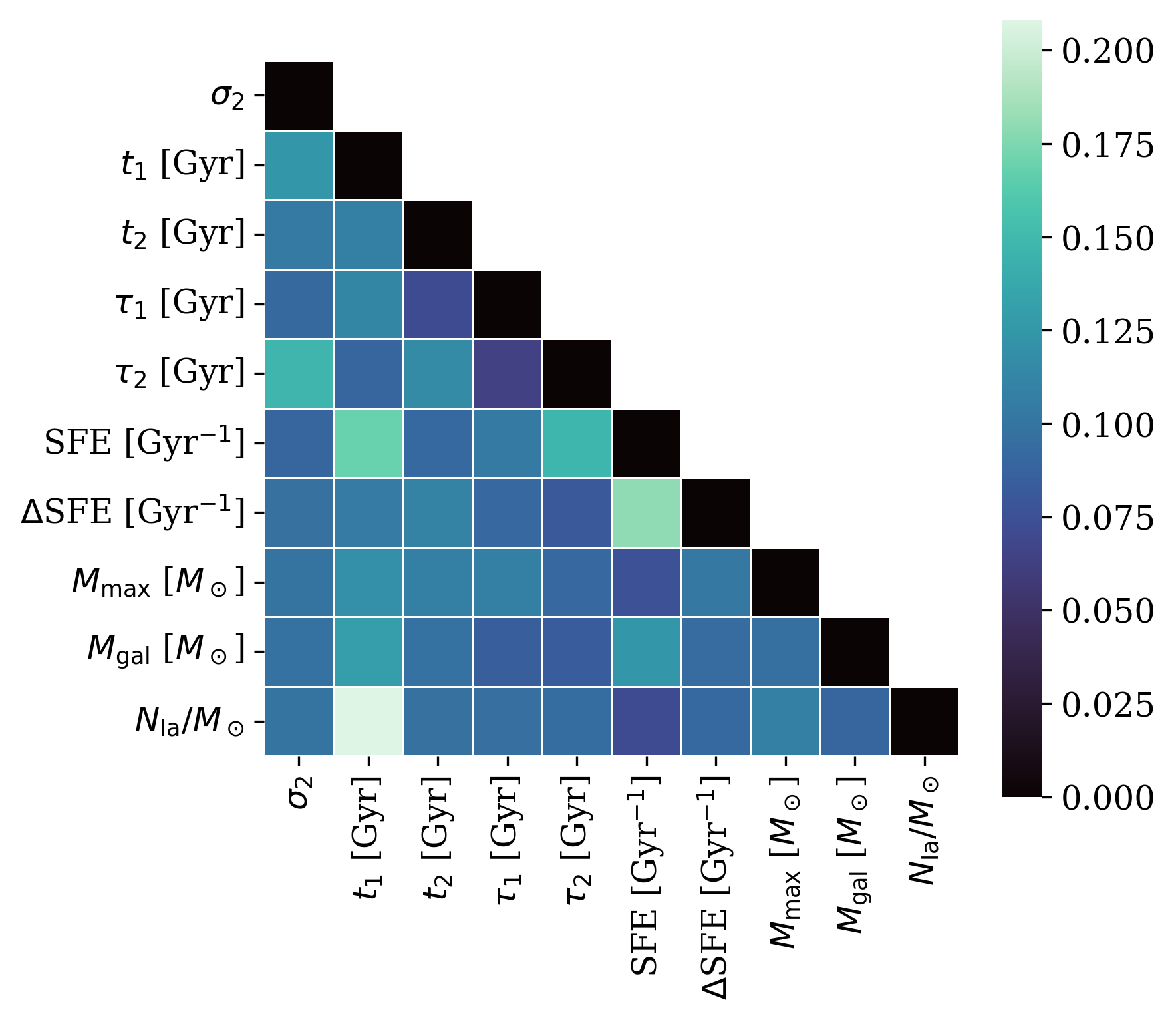
Parameter dependency analysis. \textbf{Left:
Parameter dependency analysis. \textbf{Left:
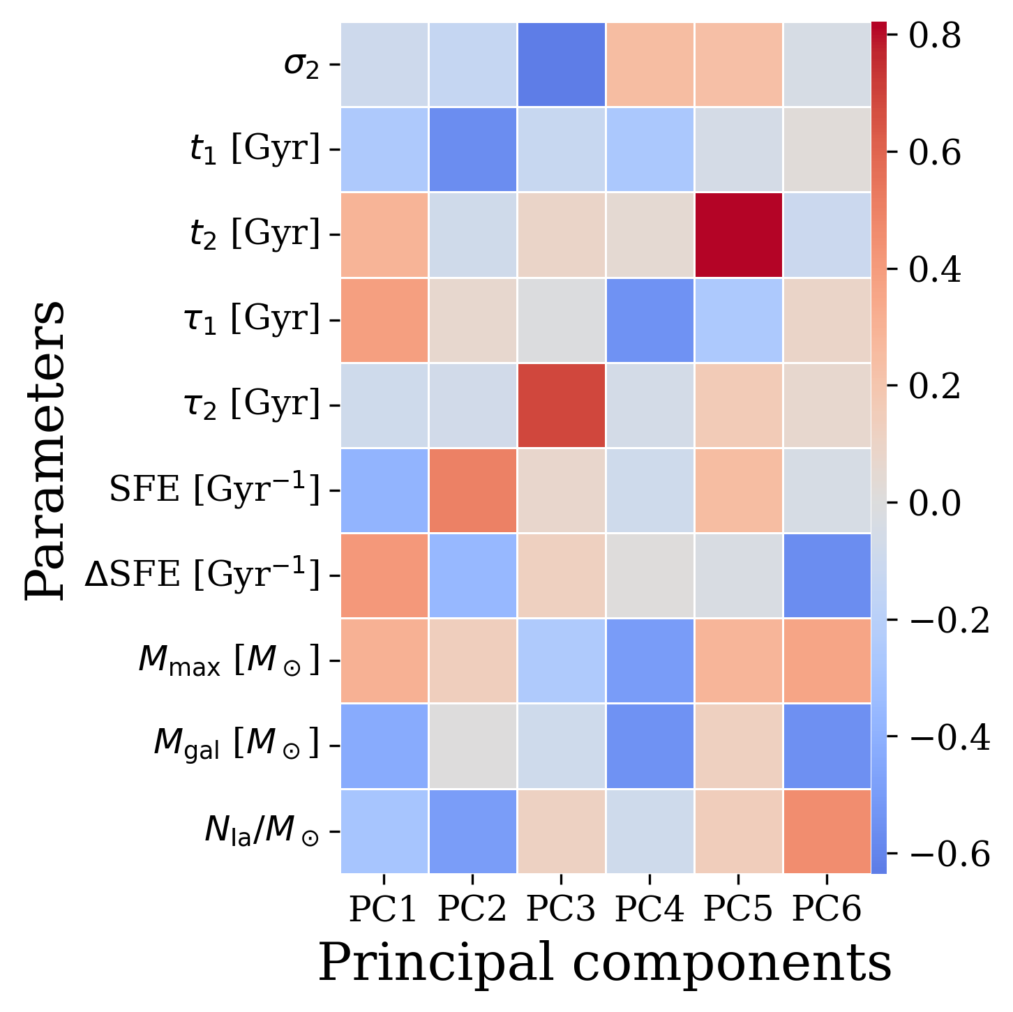
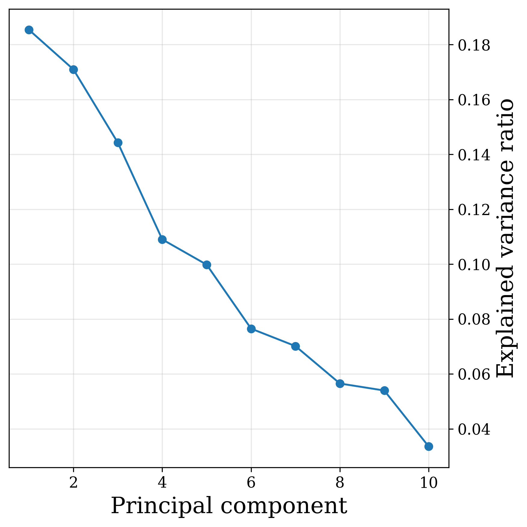
Principal component analysis of the top-performing models. \textbf{Left:
Principal component analysis of the top-performing models. \textbf{Left:
Manuscript excerpt (raw LaTeX lines)
The genetic algorithm was executed 16 times using identical hyper-parameters and prior boundaries, each starting from a different random seed.
All runs converged toward the same region of parameter space, demonstrating that the identified solution is robust and not an artifact of stochastic sampling.
The combined catalog of evaluated models was then converted into an approximate posterior-- a pseudo-posterior-- by assigning weights based on the MDF loss.
Figure~\ref{fig:param_correlations} shows the resulting pseudo-posterior distributions, which are far from Gaussian and reveal a generally broad and degenerate solution space.
Several parameters remain only weakly constrained by the MDF.
To quantify these constraints, we extract the MAP values and 68\% HDIs for all continuous parameters.
The mass ratio of the two infalls is not well constrained with maximum \textit{a posteriori} (MAP) $\sigma_2$ $\approx 0.69$ and Highest Density Interval (HDI) $0.11$--$3.1$.
The first infall time is notably more constrained than the second, where $t_1$ $\approx 0.1$~Gyr and HDI $0.09$--$0.1$~Gyr and $t_2$ $\approx 5.15$~Gyr with HDI $3.25$--$8.45$~Gyr.
The first infall timescale ($\tau_1$) is confined to a narrow range $\approx 0.09$~Gyr (HDI $0.07$--$0.10$~Gyr).
The second infall timescale is less constrained, with $\tau_2$ $\approx 1.7$~Gyr and HDI $0.5$--$3.7$~Gyr.
The SFE shows a bimodal distribution with a more prominent `high' SFE distribution (SFE $\approx 3$~Gyr$^{-1}$) and a less prominent `extremely high' SFE distribution at $\approx 25$~Gyr$^{-1}$.
Neither value is atypical when compared to previous GCE studies \citep{Matteucci09, Grieco12}.
This leads to a potentially misleading HDI of $1$--$15$~Gyr$^{-1}$.
The SN~Ia normalization ($N_{\rm Ia}/M_\odot$) is also moderately well constrained ($\approx 5.8 \times 10^{-4}$, HDI $5.0 \times 10^{-4}$--$7.9 \times 10^{-4}$).
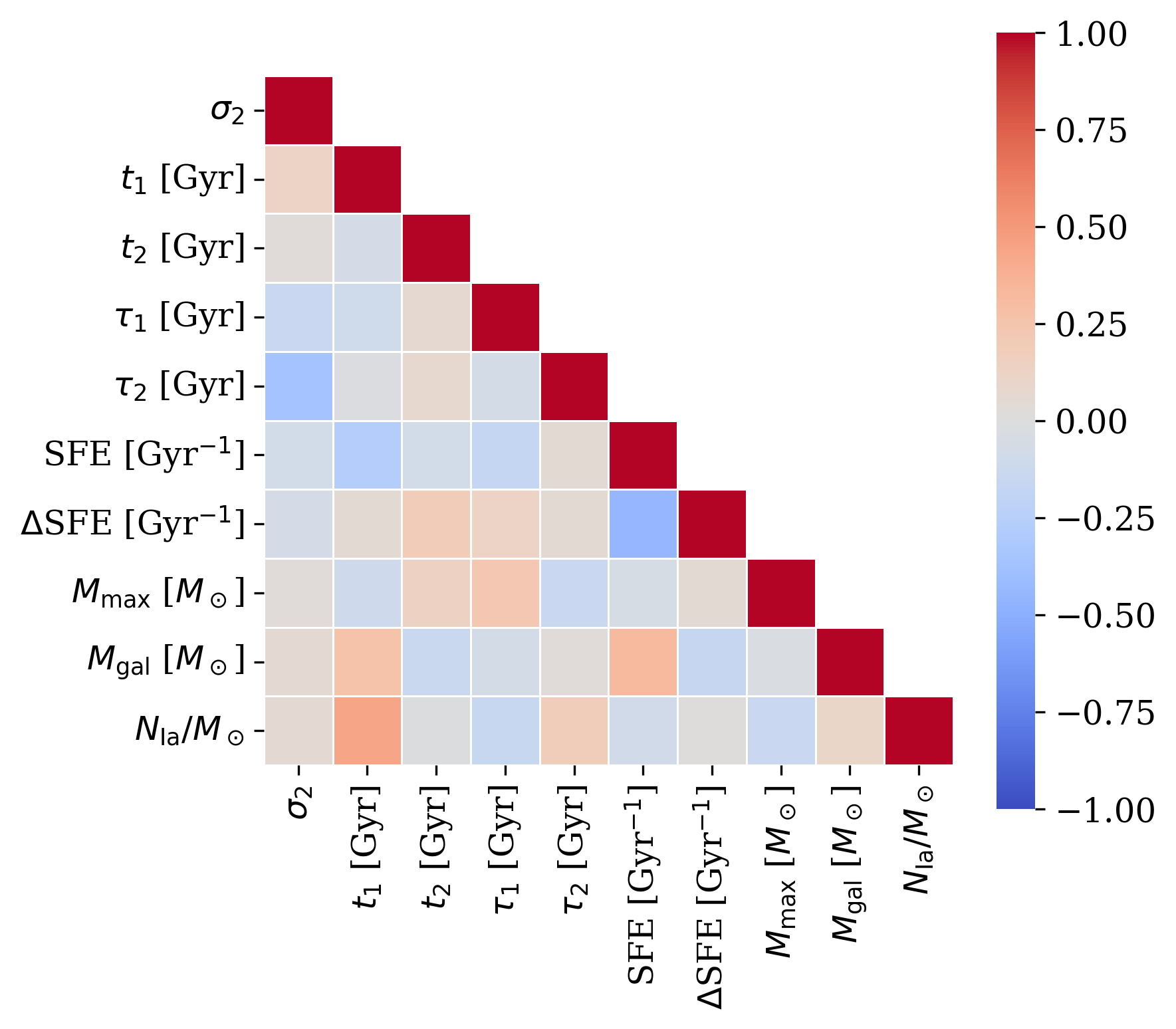
Table~\ref{tab:param_hdi_degeneracy} lists the MAP estimates and 68\% HDI for all continuous parameters, together with the strongest pairwise degeneracies.
The most pronounced linear correlation is between the infall times, timescales and the SFE, with Pearson correlation ($\rho_w$) $\simeq -0.14$ for $\tau_1$–SFE and $\rho_w \simeq -0.20$ for $t_2$–SFE (the latter being the strongest correlation in the matrix).
Parameters such as the change in SFE $\Delta\mathrm{SFE}$, the IMF upper mass $M_{\max}$, the bulge stellar mass $M_{\mathrm{Bulge}}$, and the SN~Ia normalization ($N_{\rm Ia}/M_\odot$) exhibit only modest linear correlations but large mutual information with $\sigma_2$, $\tau_1$, $\tau_2$, and $t_2$.
The pseudo-posterior exhibits several notable coupling patterns, which we describe below.
The infall mass ratio, $\sigma_2$, shows a mild negative correlation with the second–infall timescale $\tau_2$ ($\rho_w \simeq -0.18$), and both $\sigma_2$ and $\tau_2$ exhibit substantial mutual information with SFE (MI$_w \gtrsim 0.7$; Table~\ref{tab:param_hdi_degeneracy}). This indicates that the late accreted mass fraction, its delivery timescale, and the global efficiency of star formation adjust together to preserve a viable MDF. A similar negative correlation is seen between the onset time of the second infall ($t_2$) and SFE ($\rho_w \simeq -0.20$), while $\tau_2$ is negatively correlated with the first–infall timescale $\tau_1$ ($\rho_w \simeq -0.19$).
Together, these relationships produce the elongated ridges in the corner plot, corresponding to families of models in which changes to coupled parameters compensate for one another, leaving the final MDF and $\alpha$-element trends nearly unchanged.
These relationships reflect underlying physical trade-offs in bulge evolution.
Shifting gas to arrive later or over a longer timescale can be offset by adjusting the efficiency with which it is turned into stars and by redistributing mass between the first and second infall, so that the integrated enrichment history remains compatible with the present-day MDF data.
Within this credible region, the effective enrichment timescale ($\tau_{\rm enrich} \sim \tau_{\rm infall}/\nu$) remains approximately constant at $\sim 0.03$--$0.1$~Gyr, ensuring the rapid early enrichment required by the $\alpha$-knee position and the old ages of metal-poor bulge stars.
The negative correlation between $\sigma_2$ and $\tau_2$, together with their strong dependence on SFE (as quantified by the mutual information), encodes a late-time trade-off: a more massive or more concentrated second infall (higher $\sigma_2$, shorter $\tau_2$) must be compensated by a lower SFE or a shift in timing to avoid overproducing young, metal-rich stars.
In this sense, the coupled $\sigma_2$–$\tau_2$–SFE and $\tau_1$–$\tau_2$ degeneracies jointly control how aggressively the metal-rich peak of the MDF and the young end of the age–metallicity relation can be built without violating the $\alpha$-element and bulge-mass constraints.
Despite these broad individual constraints, the pseudo-posterior occupies a physically plausible region of parameter space that consistently reproduces both the observed metallicity distribution function and the \citet{Joyce2023} age–metallicity relation.
Taken together, the pseudo-posterior favors a coherent evolutionary scenario where the preferred solution describes a rapid initial collapse phase, with a first infall peaking at $t_1 \approx 0.1$~Gyr with a very short duration $\tau_1 \approx 0.1$~Gyr and an SFE of order a few~Gyr$^{-1}$.
This is followed by a delayed, lower-mass second infall episode, with onset at $t_2 \approx 5$~Gyr, corresponding to $\sim 9$~Gyr ago, with $\tau_2 \sim 1.7$~Gyr and $\sigma_2 \approx 0.69$.
This configuration naturally produces an early burst of $\alpha$-enhanced, metal-poor stars followed by a prolonged phase of diluted star formation that builds the metal-rich, younger component---exactly the hybrid classical-plus-secular scenario favored by recent bulge studies \citep{Ballero07, Takuji2012, Molero2024}.
To visualize these relationships, we compute both the weighted Pearson correlation (linear relationships among well-fitting models) and the mutual information (linear and nonlinear dependencies).
Physical Analysis
The best-fit model for the bulge indicates an extremely rapid initial star formation episode. We find that the first gas infall occurs at $t_1 \approx 0.1~\text{Gyr}$ after the birth of the Universe, with a very short infall duration of $\tau_1 \approx 0.09~\text{Gyr}$. The bulge’s primordial gas was accumulated and converted into stars on a timescale of order $10^8$ years, which is a near instantaneous collapse compared to the bulge's subsequent evolution. Such short collapse times naturally produce an early, $\alpha$-enhanced stellar population consistent with bulge age constraints.
Posterior corner plot for the continuous model parameters. Diagonal panels show 1D marginalized distributions with MAP (solid line) and 68\% highest–density intervals (dashed lines). Lower–triangle panels show the MDF–weighted model ensemble as a background point cloud with overlaid smoothed posterior density. The red crosses mark the MAP location in each 2D plane. Coloured stars and guide lines indicate parameter choices adopted in previous bulge studies, as listed in Table~\ref{tab:lit_results
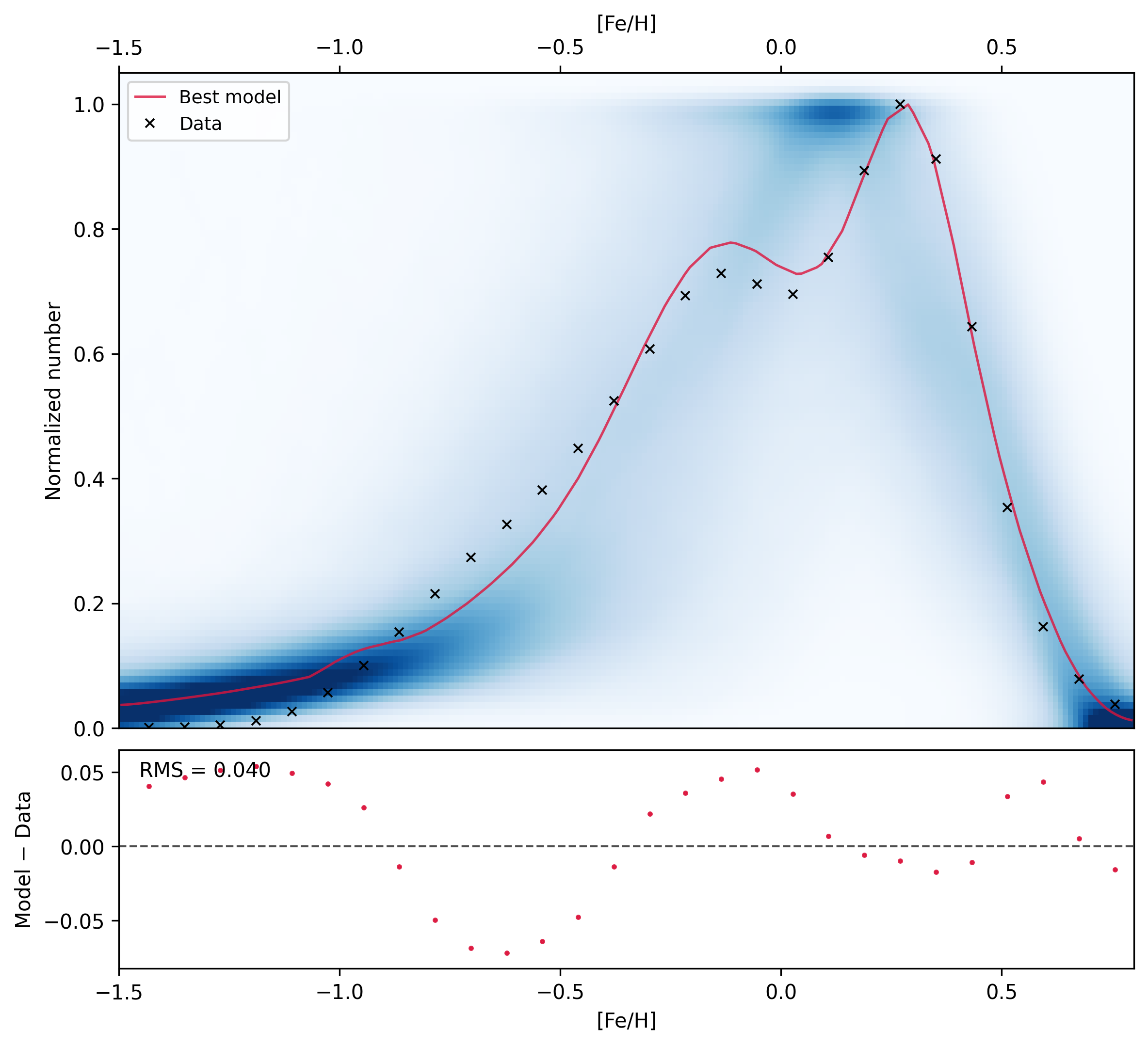
Metallicity distribution function (MDF) of the bulge for the best-fit two-infall model compared to the observed MDF. In the upper panel, the blue shading shows the posterior predictive distribution of model MDFs as a function of $\mathrm{[Fe/H]}$, the red curve marks the single best-fit model realization, and the black crosses show the empirically measured, normalized MDF. The lower panel displays the residuals (model $-$ data) for the best-fit curve in each metallicity bin, with the overall root-mean-square residual of $\mathrm{RMS}=0.040$.
Posterior [$\alpha$/Fe]–[Fe/H] relations for individual bulge $\alpha$-elements Mg, Si, Ca, and Ti for the best-fit two-infall model. In each panel, blue shading shows the posterior predictive distribution of the model abundance ratios, the red curve traces the median (best-fit) model track, and black points indicate the observed stellar abundances. The top and right insets give the corresponding one-dimensional [Fe/H] and [$\alpha$/Fe] histograms for the data (black) and model (red).
Posterior age–metallicity relation (AMR) for the bulge. The blue density field shows the weighted posterior ensemble of chemically acceptable models; the solid red line traces the MAP model. Individual stellar measurements are overplotted for comparison: \citet{Joyce2023} ages as red stars and \citet{Bensby17
Posterior age--abundance relations obtained by mapping each model’s [$\alpha$/Fe]--[Fe/H] track through the median posterior age--metallicity relation. Blue shading indicates the weighted posterior density, and the solid red curve shows the best model. Observed bulge abundances are transformed into age using the same AMR mapping and shown as black points. The panels show the intermediate-age, metal-rich population suggested by the AMR occupies the low--[$\alpha$/Fe] sequence at ages $\sim 6$--$10$~Gyr, while the oldest stars remain on the high-[$\alpha$/Fe] plateau.
Manuscript excerpt (raw LaTeX lines)
\label{sec:physical}
The best-fit model for the bulge indicates an extremely rapid initial star formation episode.
We find that the first gas infall occurs at $t_1 \approx 0.1~\text{Gyr}$ after the birth of the Universe, with a very short infall duration of $\tau_1 \approx 0.09~\text{Gyr}$.
The bulge’s primordial gas was accumulated and converted into stars on a timescale of order $10^8$ years, which is a near instantaneous collapse compared to the bulge's subsequent evolution. Such short collapse times naturally produce an early, $\alpha$-enhanced stellar population consistent with bulge age constraints.
The corresponding star formation efficiency is $\mathrm{SFE} \approx 2.93~\text{Gyr}^{-1}$ for this initial burst, which implies the gas would be largely depleted in only $\sim0.34$~Gyr ($1/\mathrm{SFE}$).
Such a high efficiency and brief timescale for the first episode are consistent with a classical rapid collapse scenario, producing a prompt enrichment of the bulge’s oldest stellar population \citep{Matteucci90}).
By contrast, the second star formation episode is significantly delayed and more prolonged.
This follows directly from the posterior’s preference for large $t_2$ and comparatively long $\tau_2$.
The model’s second infall occurs at $t_2 \approx 5.1~\text{Gyr}$, several gigayears after the initial burst, and has an extended duration of $\tau_2 \approx 1.7~\text{Gyr}$.
This delayed infall can be interpreted as a secondary gas accretion (e.g., through a merger or cooling flow) around 8.6~Gyr ago, which re-ignites star formation in the bulge.
Star formation in the second phase remains efficient but is moderately reduced relative to the initial burst.
The best-fit $\Delta_{\rm SFE} \approx 0.72$ indicates that the second-phase SFE is about 28\% lower than in the first phase.
In absolute terms, the second episode’s star formation efficiency is still on the order of $1.72~\text{Gyr}^{-1}$, sustaining rapid star formation, though not quite as extreme as the initial burst.
The inferred infall mass ratio between the two episodes is $\sigma_2 \approx 0.69$, implying that roughly 40\% of the bulge’s stellar mass formed during the second, extended episode (with the remaining $\sim60\%$ produced in the initial collapse).
This substantial later contribution helps to explain the bulge’s metal-rich population: the second infall dilutes the interstellar medium and prolongs star formation, reproducing the observed metal-rich tail of the bulge MDF. Comparisons to results from previous bulge formation models are summarized in Table~\ref{tab:lit_results}.
The literature values collected in Table \ref{tab:lit_results} reveal several systematic trends in two-infall bulge modelling which allows us to contextualize our results.
All previous studies favor a fast early bulge formation phase followed by a later episode, but our solution combines a very rapid first infall with a comparatively late and moderately extended second infall.
Our posterior supports the standard two-phase bulge picture while shifting more of the late activity to later cosmic times than most prior models.
Our first infall ($t_1 \simeq 0.1$~Gyr, $\tau_1 \simeq 0.09$~Gyr) sits at the fast end of the literature range and it is comparable to the short $\tau_1 \sim 0.1$~Gyr adopted by \citet{Grieco12}, \citet{Molero2024}, and \citet{Ballero07}.
The second episode in our model begins later ($t_2 \simeq 5.1$~Gyr) than in \citet{Grieco12} ($t_2 \sim 2$~Gyr), with an intermediate timescale ($\tau_2 \simeq 1.7$~Gyr, between the $\sim 1.5$–3~Gyr used by \citealt{Grieco12, Nieuwmunster23}, and \citet{Takuji2012}
Our inferred mass ratio ($\sigma_2 \simeq 0.69$) implies that the second episode contributes $\sim 40\%$ of the bulge mass, intermediate between the smaller late contribution assumed by \citet{Molero2024} ($\sigma_2 \simeq 0.4$).
Our SFEs (SFE$_1 \simeq 2.9$~Gyr$^{-1}$ and SFE$_2 \simeq 2.1$~Gyr$^{-1}$) are high but well below the very intense bursts (SFE $\sim 20$–25~Gyr$^{-1}$) adopted by \citet{Grieco12}, \citet{Molero2024}, and \citet{Matteucci19}.
Our bulge stellar mass ($M_{\mathrm{Bulge}} \simeq 1.0\times 10^{10}\,M_\odot$) and SN\,Ia rate per unit mass ($N_{\rm Ia}/M_\odot \simeq 5.8\times 10^{-4}$) fall toward the lower end of the ranges assumed in previous studies.
For example, \citet{Grieco12} adopt $M_{\mathrm{Bulge}} \sim 2\times 10^{10}\,M_\odot$ and $N_{\rm Ia}/M_\odot \sim 10^{-3}$, while our values are closer to the $M_{\mathrm{Bulge}} \sim 10^{10}\,M_\odot$ used by \citet{Molero2024}.
\subsection{The Metallicity Distribution Function}% \mj{[This section is unfinished]}}
\vspace{0.2cm}
Figure \ref{fig:mdf-fit} shows how the posterior ensemble of models compares to the observed MDF.
Best-fit two-infall models successfully recover the observed metallicity distribution function with high fidelity, achieving an RMS residual of $0.040$.
The MDF encodes the integrated enrichment history of the bulge, so matching its shape is the primary aim of this study.
The models capture both the characteristic near-solar metallicity peak and the extended metal-poor tail that defines the bulge population.
Conclusions
A two-infall chemical evolution model suggest that the first infall episode occurs rapidly ($t_1 \approx 0.1$ Gyr, $\tau_1 \approx 0.09$ Gyr), forming $\sim60$\% of the bulge mass with high SFE ($\sim 2.9$ Gyr$^{-1}$), consistent with a classical collapse and the second infall episode is delayed ($t_2 \approx 5.1$ Gyr, $\tau_2 \approx 1.7$ Gyr) and moderately extended, contributing $\sim40$\% of the stellar mass with reduced SFE ($\sim 2.1$ Gyr$^{-1}$). We find that the second infall is chemically required to produce the super-solar MDF peak and the low-[$\alpha$/Fe] population; models without a non-zero second episode cannot fit the data, even in the presence of degeneracies among $\sigma_2$, $t_2$, $\tau_2$, and $\Delta$SFE. Lower SFE and longer $\tau_2$ during this phase allow extended iron enrichment from SNe~Ia, generating the observed [$\alpha$/Fe] downturn. In this framework the first episode explains the $\alpha$-enhanced, metal-poor population, while the delayed second episode builds the younger, metal-rich tail and simultaneously reproduces the MDF bimodality, the [$\alpha$/Fe] knee position, and the Joyce–Johnson AMR without imposing direct age constraints.
Manuscript excerpt (raw LaTeX lines)
A two-infall chemical evolution model suggest that the first infall episode occurs rapidly ($t_1 \approx 0.1$ Gyr, $\tau_1 \approx 0.09$ Gyr), forming $\sim60$\% of the bulge mass with high SFE ($\sim 2.9$ Gyr$^{-1}$), consistent with a classical collapse and the second infall episode is delayed ($t_2 \approx 5.1$ Gyr, $\tau_2 \approx 1.7$ Gyr) and moderately extended, contributing $\sim40$\% of the stellar mass with reduced SFE ($\sim 2.1$ Gyr$^{-1}$).
\textbf{Using OMEGA++ with a genetic algorithm to explore a 15-dimensional parameter space our model reproduces the bulge's MDF, AMR, and alpha-element patterns with high fidelity.}
We find that the second infall is chemically required to produce the super-solar MDF peak and the low-[$\alpha$/Fe] population; models without a non-zero second episode cannot fit the data, even in the presence of degeneracies among $\sigma_2$, $t_2$, $\tau_2$, and $\Delta$SFE. Lower SFE and longer $\tau_2$ during this phase allow extended iron enrichment from SNe~Ia, generating the observed [$\alpha$/Fe] downturn.
In this framework the first episode explains the $\alpha$-enhanced, metal-poor population, while the delayed second episode builds the younger, metal-rich tail and simultaneously reproduces the MDF bimodality, the [$\alpha$/Fe] knee position, and the Joyce–Johnson AMR without imposing direct age constraints.
Residual tensions remain with the super-solar ages and Ti abundances reported by \citet{Bensby17}, highlighting the need for improved stellar models and age determinations.
PCA and mutual-information analyses show that several parameter combinations can preserve the MDF and [$\alpha$/Fe] trends, and that categorical choices (IMF, yield set, SN~Ia implementation) are not uniquely determined but are largely absorbed through compensating shifts in the continuous parameters.
Even so, the requirement for two distinct infall episodes is robust, and the recovered SFE values are high but sub-bursting, lower than the 20–25~Gyr$^{-1}$ assumed in some previous bulge models and more consistent with modern observational constraints.
The bulge likely formed in a hybrid scenario: early rapid collapse followed by moderate secular or merger-driven gas inflow, without requiring a third distinct episode.
Limitations include the one-zone assumption, fixed yields, lack of dynamics, and no explicit modeling of radial migration or spatial gradients.
However, despite simplifications, the two-infall + reduced-SFE model reproduces all key observables and provides a coherent, physically motivated picture of bulge formation.
This study demonstrates the Milky Way bulge as a critical laboratory for disentangling the relationship between rapid high-redshift collapse and prolonged secular evolution in spiral galaxies.
Our results demonstrate that reproducing the chemical profile of the bulge is attainable through a hybrid formation history.
These chemical constraints provide a benchmark for future work, which must move beyond one-zone approximations to spatially resolved chemodynamical simulations capable of capturing radial and vertical gradients.
Future Work
A number of forthcoming observational advances and modeling improvements could significantly strengthen the constraints on bulge-formation scenarios and help discriminate between competing hypotheses. First, new and upcoming surveys such as the Nancy Grace Roman Space Telescope Galactic Bulge Time-Domain Survey (GBTDS) will provide deep, high-cadence near-infrared photometry --- including grism spectroscopy ``snapshots'' --- for hundreds of millions of stars in the bulge region \citep{Gaudi2022}. These data will enable asteroseismic age estimates for large samples of red-giant stars \citep{Huber2023, Weiss2025}, and more robust metallicity and kinematic measurements, thereby providing far more precise MDFs and abundance-age distributions than currently possible.
Manuscript excerpt (raw LaTeX lines)
A number of forthcoming observational advances and modeling improvements could significantly strengthen the constraints on bulge-formation scenarios and help discriminate between competing hypotheses.
First, new and upcoming surveys such as the Nancy Grace Roman Space Telescope Galactic Bulge Time-Domain Survey (GBTDS) will provide deep, high-cadence near-infrared photometry --- including grism spectroscopy ``snapshots'' --- for hundreds of millions of stars in the bulge region \citep{Gaudi2022}.
These data will enable asteroseismic age estimates for large samples of red-giant stars \citep{Huber2023, Weiss2025}, and more robust metallicity and kinematic measurements, thereby providing far more precise MDFs and abundance-age distributions than currently possible.
Combined with long-time baseline surveys such as the Vera C. Rubin Observatory Legacy Survey of Space and Time (LSST), the joint optical and near-IR coverage will more effectively pierce dust extinction (with LSST reaching single-visit depths of $\sim24–25$~mag in the optical bands and up to $\sim27$~mag in the 10-yr coadds) and crowding toward the Galactic center (with a pixel scale of $0.2''$~per~pixel), increasing completeness and stellar sampling depth \citep{Street2018, Gonzalez2018}.\looseness-1
A spatially resolved approach to modeling the bulge --- splitting the bulge volume into multiple zones (e.g.\ by galactocentric radius and/or latitudinal binning) --- would allow the reconstruction of radial and vertical metallicity gradients, localized enrichment episodes, and possible structural subpopulations.
Observational metallicity-maps like those derived from the VVV Survey and 2MASS photometry already show clear vertical metallicity gradients across the bulge \citep{Gonzalez2013,Ness2016, Johnson2022}.
Also, integrating chemical evolution modeling with dynamical or hydrodynamical simulations --- allowing gas flows, radial mixing, bar-induced inflows, and non-instantaneous mixing --- will yield more realistic predictions for the bulge’s chemical and structural evolution.  Such models will be essential to predict and compare spatial abundance gradients, alpha-element substructures, and age–metallicity relations as a function of position in the bulge.  Furthermore, combined chemical and hydrodynamical modeling will be important for deciphering the role bar formation timing plays in chemical enrichment.  The results presented here indicate a majority mass fraction forming at very early times, likely before the bar.  However, the slowly rotating, high velocity component of the bulge is found to be relatively small \citep{Kunder16, Arentsen20} while a majority of bulge stars exhibit bar-like kinematics \citep[e.g.,][]{Kunder12, Marchetti24}.  We expect that a combined approach will yield deeper insight into reconciling the interplay between chemistry and kinematics.
\begin{acknowledgments}
The authors wish to thank the University of Wyoming Advanced Research Computing Center (ARCC).
N. Miller wishes to thank Katherine Miller for Figure~\ref{fig:intro-cartoon}.
M. Joyce wishes to thank John Bourke for typsetting.
This manuscript made use of the NASA ADS library.
\end{acknowledgments}
\software{OMEGA+, Python, numpy, DEMC, pandas, BASH, LaTeX, ChatGPT, Gemini}
\bibliography{all_bib}
\bibliographystyle{aasjournal}
\appendix
Validation of Genetic Algorithms with DEMC against Classical MCMC
We ran an MCMC for each unique set of catagorical parameters (outlined in Table \ref{tab:parameter_space}) and combined their posteriors. To check whether the GA with DEMC moves is sampling the same posterior as a conventional MCMC, we repeated the analysis with independent MCMC runs and compared the resulting posteriors. For every distinct choice of categorical parameters we launched a separate MCMC run in the continuous parameters.
Corner plot of the joint posterior distribution in the continuous two–infall parameters obtained by combining 288 independent MCMC runs, one for each unique choice of categorical model ingredients Table~\ref{tab:parameter_space
Manuscript excerpt (raw LaTeX lines)
We ran an MCMC for each unique set of catagorical parameters (outlined in Table \ref{tab:parameter_space}) and combined their posteriors.
To check whether the GA with DEMC moves is sampling the same posterior as a conventional MCMC, we repeated the analysis with independent MCMC runs and compared the resulting posteriors.
For every distinct choice of categorical parameters we launched a separate MCMC run in the continuous parameters.
Each run used the same likelihood, priors, and parameter ranges as in the GA+DEMC analysis.
After discarding an initial burn-in segment, the chains were concatenated over all categorical combinations.
The resulting catalogue of MCMC samples was weighted in exactly the same way as the GA+DEMC models (using the MDF-based loss) and converted into a posterior.
From this combined MCMC posterior we computed the same summary statistics as in the main text: MAP estimates and 68\% HDI limits for each parameter, and pairwise degeneracy metrics.
The one–dimensional MCMC marginals agree with the GA+DEMC results to within the sampling noise, and the same dominant degeneracies appear in the 2D projections.
Visually, the MCMC corner plot in Figure~\ref{fig:placeholder} is similar to the GA+DEMC posterior shown in Figure~\ref{fig:param_correlations}, and the MAP/HDI numbers in Table~\ref{tab:param_hdi_degeneracy} are reproduced by the MCMC chains.
Table~\ref{tab:ga_mcmc_cost} summarizes the computational cost of the GA+DEMC and MCMC approaches.
This demonstrates that the GA with DEMC moves is tracing the same posterior distribution as a standard MCMC.
Convergence Testing
We assess GA convergence by tracking the 68\% highest–posterior–density (HPD) size of key two–parameter projections as a function of generation. For each generation, we compute the semi–major axis of the weighted covariance ellipse in the $(\sigma_2,t_2)$, $(t_1,t_2)$, $(\tau_1,t_2)$, $(\tau_2,t_2)$, and $(\tau_1,\tau_2)$ planes using the top–weighted models from a single GA run (solid curves). As shown in Figure~\ref{fig:hpd_convergence}, the 68\% HPD ellipse sizes shrink rapidly in early generations and then plateau, indicating stable convergence of the GA.
Convergence of the GA posterior. Solid lines show the evolution of the 68\% HPD ellipse size for several parameter pairs as a function of generation for a single GA run. Dotted lines show the corresponding HPD sizes measured from the combined pseudo–posterior used in the main corner plot. The rapid early decrease and subsequent plateau, together with the close agreement between solid and dotted curves, indicate stable and repeatable convergence of the GA.
Manuscript excerpt (raw LaTeX lines)
We assess GA convergence by tracking the 68\% highest–posterior–density (HPD) size of key two–parameter projections as a function of generation.
For each generation, we compute the semi–major axis of the weighted covariance ellipse in the $(\sigma_2,t_2)$, $(t_1,t_2)$, $(\tau_1,t_2)$, $(\tau_2,t_2)$, and $(\tau_1,\tau_2)$ planes using the top–weighted models from a single GA run (solid curves).
As shown in Figure~\ref{fig:hpd_convergence}, the 68\% HPD ellipse sizes shrink rapidly in early generations and then plateau, indicating stable convergence of the GA.
The HPD sizes shrink rapidly in the early generations and then flatten, indicating that the GA transitions from exploration to local refinement rather than continuing to discover new regions of parameter space.
A second set of curves (dotted lines) shows the same HPD sizes measured from the combined pseudo–posterior used to build the main corner plot in the text (i.e.\ all GA+DEMC runs together). The dotted curves closely track the solid curves at late generations.
The agreement between single–run HPD sizes and the combined posterior, together with the monotonic shrinkage and saturation of the HPD envelopes, demonstrates that independent GA realizations converge reliably and consistently to the same region of parameter space.
\end{document}